6.16. DataFrame Statistics
.count().value_counts().nunique().sum().cumsum().prod().cumprod().min().idxmin().cummin().max().idxmax().cummax().mean().median().mode().rolling(window=3).mean().abs().std().mad()- Mean absolute deviation (PL: Odchylenie bezwzględne).sem()- Standard Error of the Mean (SEM) (PL: błąd standardowy średniej).skew()- Skewness - 3rd moment (PL: skośność).kurt()- Kurtosis - 4th moment (PL: kurtoza).quantile(.33)- Sample quantile (value at %). Quantile also known as Percentile.quantile([.25, .5, .75]).var().corr().describe().nsmallest().values().rank()- Compute numerical data ranks (1 through n) along axis.
6.16.1. SetUp
>>> import pandas as pd
>>> import numpy as np
>>> np.random.seed(0)
>>>
>>>
>>> df = pd.DataFrame(
...     columns = ['Morning', 'Noon', 'Evening', 'Midnight'],
...     index = pd.date_range('1999-12-30', periods=7),
...     data = np.random.randn(7, 4))
>>>
>>> df
             Morning      Noon   Evening  Midnight
1999-12-30  1.764052  0.400157  0.978738  2.240893
1999-12-31  1.867558 -0.977278  0.950088 -0.151357
2000-01-01 -0.103219  0.410599  0.144044  1.454274
2000-01-02  0.761038  0.121675  0.443863  0.333674
2000-01-03  1.494079 -0.205158  0.313068 -0.854096
2000-01-04 -2.552990  0.653619  0.864436 -0.742165
2000-01-05  2.269755 -1.454366  0.045759 -0.187184
6.16.2. Count
Number of non-null observations:
>>> df.count()
Morning     7
Noon        7
Evening     7
Midnight    7
dtype: int64
>>> df.value_counts()
Morning    Noon       Evening   Midnight
 1.764052   0.400157  0.978738   2.240893    1
 1.867558  -0.977278  0.950088  -0.151357    1
-0.103219   0.410599  0.144044   1.454274    1
 0.761038   0.121675  0.443863   0.333674    1
 1.494079  -0.205158  0.313068  -0.854096    1
-2.552990   0.653619  0.864436  -0.742165    1
 2.269755  -1.454366  0.045759  -0.187184    1
Name: count, dtype: int64
>>> df.nunique()
Morning     7
Noon        7
Evening     7
Midnight    7
dtype: int64
6.16.3. Sum
Sum of values:
df.sum() Morning 5.500273 Noon -1.050752 Evening 3.739996 Midnight 2.094039 dtype: float64
Cumulative sum:
>>> df.cumsum()
             Morning      Noon   Evening  Midnight
1999-12-30  1.764052  0.400157  0.978738  2.240893
1999-12-31  3.631610 -0.577121  1.928826  2.089536
2000-01-01  3.528391 -0.166522  2.072870  3.543809
2000-01-02  4.289429 -0.044847  2.516733  3.877484
2000-01-03  5.783508 -0.250005  2.829801  3.023388
2000-01-04  3.230518  0.403613  3.694237  2.281223
2000-01-05  5.500273 -1.050752  3.739996  2.094039
6.16.4. Product
Product of values:
>>> df.prod()
Morning     2.240538
Noon       -0.003810
Evening     0.000736
Midnight    0.019528
dtype: float64
Cumulative product:
>>> df.cumprod()
             Morning      Noon   Evening  Midnight
1999-12-30  1.764052  0.400157  0.978738  2.240893
1999-12-31  3.294470 -0.391065  0.929888 -0.339175
2000-01-01 -0.340051 -0.160571  0.133944 -0.493254
2000-01-02 -0.258792 -0.019537  0.059453 -0.164586
2000-01-03 -0.386656  0.004008  0.018613  0.140572
2000-01-04  0.987128  0.002620  0.016090 -0.104328
2000-01-05  2.240538 -0.003810  0.000736  0.019528
6.16.5. Extremes
Minimum, index of minimum and cumulative minimum:
>>> df.min()
Morning    -2.552990
Noon       -1.454366
Evening     0.045759
Midnight   -0.854096
dtype: float64
>>> df.idxmin()
Morning    2000-01-04
Noon       2000-01-05
Evening    2000-01-05
Midnight   2000-01-03
dtype: datetime64[us]
>>> df.cummin()
             Morning      Noon   Evening  Midnight
1999-12-30  1.764052  0.400157  0.978738  2.240893
1999-12-31  1.764052 -0.977278  0.950088 -0.151357
2000-01-01 -0.103219 -0.977278  0.144044 -0.151357
2000-01-02 -0.103219 -0.977278  0.144044 -0.151357
2000-01-03 -0.103219 -0.977278  0.144044 -0.854096
2000-01-04 -2.552990 -0.977278  0.144044 -0.854096
2000-01-05 -2.552990 -1.454366  0.045759 -0.854096
Maximum, index of maximum and cumulative maximum:
>>> df.max()
Morning     2.269755
Noon        0.653619
Evening     0.978738
Midnight    2.240893
dtype: float64
>>> df.idxmax()
Morning    2000-01-05
Noon       2000-01-04
Evening    1999-12-30
Midnight   1999-12-30
dtype: datetime64[us]
>>> df.cummax()
             Morning      Noon   Evening  Midnight
1999-12-30  1.764052  0.400157  0.978738  2.240893
1999-12-31  1.867558  0.400157  0.978738  2.240893
2000-01-01  1.867558  0.410599  0.978738  2.240893
2000-01-02  1.867558  0.410599  0.978738  2.240893
2000-01-03  1.867558  0.410599  0.978738  2.240893
2000-01-04  1.867558  0.653619  0.978738  2.240893
2000-01-05  2.269755  0.653619  0.978738  2.240893
6.16.6. Average
Arithmetic mean of values:
>>> df.mean()
Morning     0.785753
Noon       -0.150107
Evening     0.534285
Midnight    0.299148
dtype: float64
Arithmetic median of values:
>>> df.median()
Morning     1.494079
Noon        0.121675
Evening     0.443863
Midnight   -0.151357
dtype: float64
Mode:
>>> df.mode()
    Morning      Noon   Evening  Midnight
0 -2.552990 -1.454366  0.045759 -0.854096
1 -0.103219 -0.977278  0.144044 -0.742165
2  0.761038 -0.205158  0.313068 -0.187184
3  1.494079  0.121675  0.443863 -0.151357
4  1.764052  0.400157  0.864436  0.333674
5  1.867558  0.410599  0.950088  1.454274
6  2.269755  0.653619  0.978738  2.240893
Rolling Average:
>>> df.rolling(window=30)
Rolling [window=30,center=False,method=single]
>>>
>>> df.rolling(window=3).mean()
             Morning      Noon   Evening  Midnight
1999-12-30       NaN       NaN       NaN       NaN
1999-12-31       NaN       NaN       NaN       NaN
2000-01-01  1.176130 -0.055507  0.690957  1.181270
2000-01-02  0.841792 -0.148335  0.512665  0.545530
2000-01-03  0.717299  0.109038  0.300325  0.311284
2000-01-04 -0.099291  0.190045  0.540456 -0.420862
2000-01-05  0.403615 -0.335302  0.407754 -0.594482
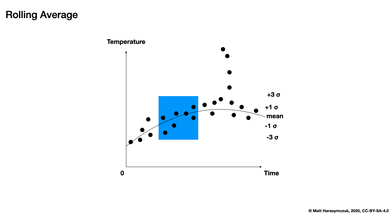
Figure 6.11. Rolling Average
6.16.7. Distribution
Absolute value:
>>> df.abs()
             Morning      Noon   Evening  Midnight
1999-12-30  1.764052  0.400157  0.978738  2.240893
1999-12-31  1.867558  0.977278  0.950088  0.151357
2000-01-01  0.103219  0.410599  0.144044  1.454274
2000-01-02  0.761038  0.121675  0.443863  0.333674
2000-01-03  1.494079  0.205158  0.313068  0.854096
2000-01-04  2.552990  0.653619  0.864436  0.742165
2000-01-05  2.269755  1.454366  0.045759  0.187184
Standard deviation:
>>> df.std()
Morning     1.671798
Noon        0.787967
Evening     0.393169
Midnight    1.151785
dtype: float64
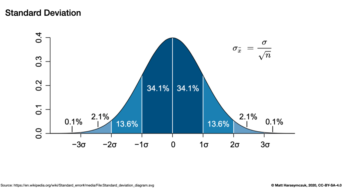
Figure 6.12. Standard Deviation
Standard Error of the Mean (SEM):
>>> df.sem()
Morning     0.631880
Noon        0.297824
Evening     0.148604
Midnight    0.435334
dtype: float64
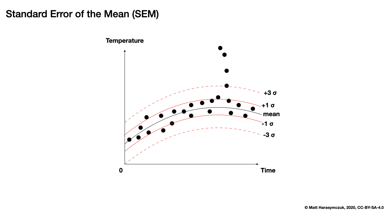
Figure 6.13. Standard Error of the Mean (SEM)
Skewness (3rd moment):
>>> df.skew()
Morning    -1.602706
Noon       -0.907414
Evening     0.031047
Midnight    0.915190
dtype: float64
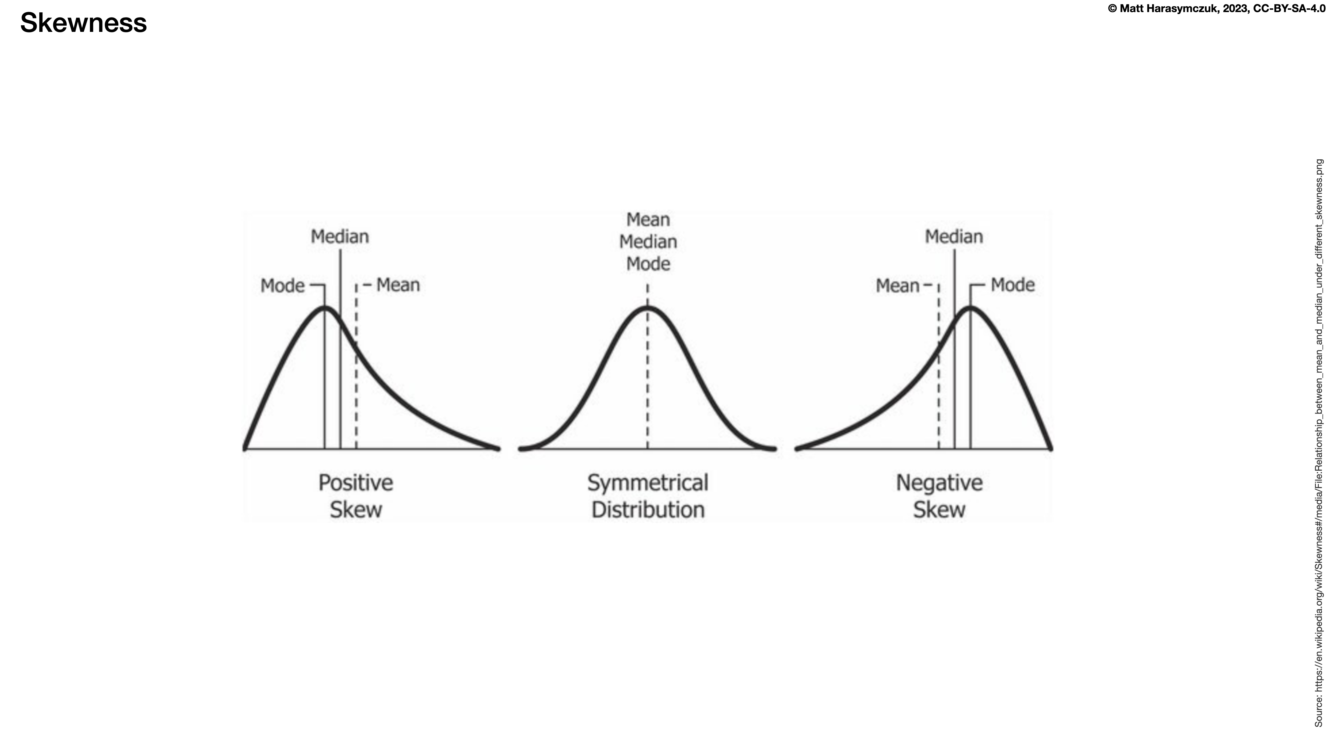
Figure 6.14. Skewness
Kurtosis (4th moment):
>>> df.kurt()
Morning     2.502051
Noon       -0.588010
Evening    -2.208781
Midnight   -0.351782
dtype: float64
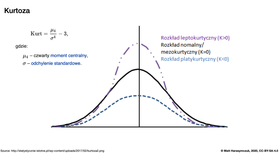
Figure 6.15. Kurtosis
Sample quantile (value at %). Quantile also known as Percentile:
>>> df.quantile(.33)
Morning     0.743753
Noon       -0.220601
Evening     0.309687
Midnight   -0.198283
Name: 0.33, dtype: float64
>>> df.quantile([.25, .5, .75])
       Morning      Noon   Evening  Midnight
0.25  0.328909 -0.591218  0.228556 -0.464674
0.50  1.494079  0.121675  0.443863 -0.151357
0.75  1.815805  0.405378  0.907262  0.893974
Variance:
>>> df.var()
Morning     2.794907
Noon        0.620892
Evening     0.154582
Midnight    1.326610
dtype: float64
Correlation Coefficient:
>>> df.corr()
           Morning      Noon   Evening  Midnight
Morning   1.000000 -0.698340 -0.190219  0.201034
Noon     -0.698340  1.000000  0.307686  0.359761
Evening  -0.190219  0.307686  1.000000  0.136436
Midnight  0.201034  0.359761  0.136436  1.000000
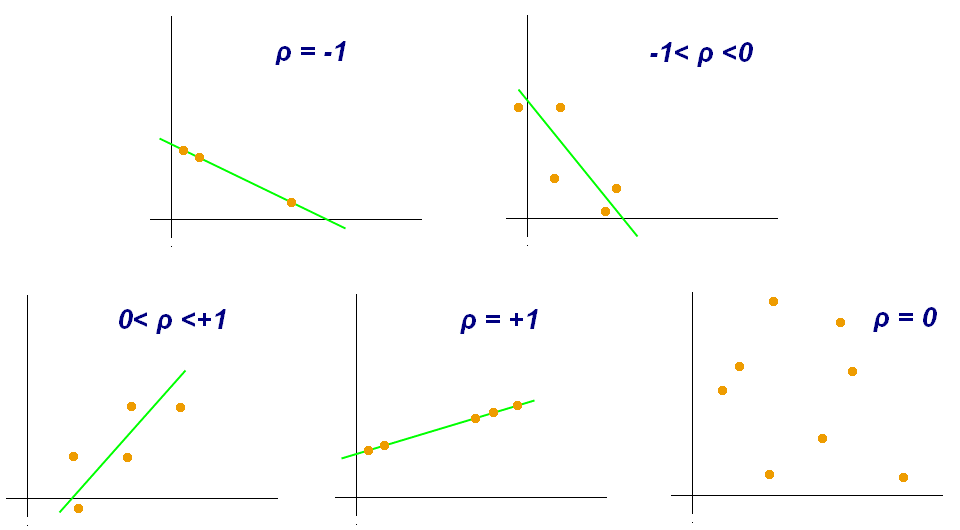
Figure 6.16. Correlation Coefficient
6.16.8. Describe
>>> df.describe()
        Morning      Noon   Evening  Midnight
count  7.000000  7.000000  7.000000  7.000000
mean   0.785753 -0.150107  0.534285  0.299148
std    1.671798  0.787967  0.393169  1.151785
min   -2.552990 -1.454366  0.045759 -0.854096
25%    0.328909 -0.591218  0.228556 -0.464674
50%    1.494079  0.121675  0.443863 -0.151357
75%    1.815805  0.405378  0.907262  0.893974
max    2.269755  0.653619  0.978738  2.240893
6.16.9. Examples
>>> import pandas as pd
>>>
>>>
>>> DATA = 'https://python3.info/_static/phones-en.csv'
>>>
>>> df = pd.read_csv(DATA, parse_dates=['date'])
>>> df.drop(columns='index', inplace=True)
- date
The date and time of the entry
- duration
The duration (in seconds) for each call, the amount of data (in MB) for each data entry, and the number of texts sent (usually 1) for each sms entry
- item
A description of the event occurring – can be one of call, sms, or data
- month
The billing month that each entry belongs to – of form
YYYY-MM- network
The mobile network that was called/texted for each entry
- network_type
Whether the number being called was a mobile, international ('world'), voicemail, landline, or other ('special') number.
Source [1]
How many rows the dataset:
>>> df['item'].count()
np.int64(830)
What was the longest phone call / data entry?:
>>> df['duration'].max()
np.float64(10528.0)
How many seconds of phone calls are recorded in total?:
>>> df.loc[ df['item'] == 'call' ]['duration'].sum()
np.float64(92321.0)
How many entries are there for each month?:
>>> df['month'].value_counts()
month
2014-11    230
2015-01    205
2014-12    157
2015-02    137
2015-03    101
Name: count, dtype: int64
Number of non-null unique network entries:
>>> df['network'].nunique()
9
6.16.10. Other
.nsmallest()
.values()
.rank()
6.16.11. References
6.16.12. Assignments
# %% About
# - Name: DataFrame Statistics
# - Difficulty: medium
# - Lines: 1
# - Minutes: 2

# %% License
# - Copyright 2025, Matt Harasymczuk <matt@python3.info>
# - This code can be used only for learning by humans
# - This code cannot be used for teaching others
# - This code cannot be used for teaching LLMs and AI algorithms
# - This code cannot be used in commercial or proprietary products
# - This code cannot be distributed in any form
# - This code cannot be changed in any form outside of training course
# - This code cannot have its license changed
# - If you use this code in your product, you must open-source it under GPLv2
# - Exception can be granted only by the author

# %% English
# 1. Save basic descriptive statistics to `result: pd.DataFrame`
# 2. Run doctests - all must succeed

# %% Polish
# 1. Zapisz podstawowe statystyki opisowe do `result: pd.DataFrame`
# 2. Uruchom doctesty - wszystkie muszą się powieść

# %% Expected
# >>> result  # doctest: +NORMALIZE_WHITESPACE
#            mileage  consumption
# count      50.0000      50.0000
# mean   110421.0200       9.3200
# std     53170.2433       6.2448
# min      7877.0000       0.0000
# 25%     71239.7500       4.0000
# 50%    115186.0000       9.0000
# 75%    154889.0000      14.7500
# max    199827.0000      20.0000

# %% Hints
# - `DataFrame.describe()`

# %% Doctests
"""
>>> import sys; sys.tracebacklimit = 0

>>> assert sys.version_info >= (3, 9), \
'Python has an is invalid version; expected: `3.9` or newer.'

>>> pd.set_option('display.width', 500)
>>> pd.set_option('display.max_columns', 10)
>>> pd.set_option('display.max_rows', 10)
>>> pd.set_option('display.precision', 4)

>>> assert 'result' in globals(), \
'Variable `result` is not defined; assign result of your program to it.'

>>> assert result is not Ellipsis, \
'Variable `result` has an invalid value; assign result of your program to it.'

>>> assert type(result) is pd.DataFrame, \
'Variable `result` has an invalid type; expected: `pd.DataFrame`.'

>>> result  # doctest: +NORMALIZE_WHITESPACE
           mileage  consumption
count      50.0000      50.0000
mean   110421.0200       9.3200
std     53170.2433       6.2448
min      7877.0000       0.0000
25%     71239.7500       4.0000
50%    115186.0000       9.0000
75%    154889.0000      14.7500
max    199827.0000      20.0000
"""

# %% Run
# - PyCharm: right-click in the editor and `Run Doctest in ...`
# - PyCharm: keyboard shortcut `Control + Shift + F10`
# - Terminal: `python -m doctest -f -v myfile.py`

# %% Imports
import pandas as pd
import numpy as np

# %% Types
result: pd.DataFrame

# %% Data
np.random.seed(0)

df = pd.DataFrame({
    'mileage': np.random.randint(0, 200_000, size=50),
    'consumption': np.random.randint(0, 21, size=50),
})

# %% Result
result = ...