4.11. Series Statistics

4.11.1. SetUp

>>> import pandas as pd
>>> import numpy as np
>>>
>>>
>>> s = pd.Series(
...     data = [1.0, 2.0, 3.0, np.nan, 5.0],
...     index = ['a', 'b', 'c', 'd', 'e'])
>>>
>>> s
a    1.0
b    2.0
c    3.0
d    NaN
e    5.0
dtype: float64

4.11.2. Count

• Series.count() - Number of non-null observations

>>> len(s)
5
>>> s.size
5
>>> s.count()
4
>>> s.nunique()
4

>>> s.value_counts()
1.0    1
2.0    1
3.0    1
5.0    1
Name: count, dtype: int64

4.11.3. Sum

• Series.sum() - Sum of values

• Series.cumsum() - Cumulative sum

>>> s.sum()
11.0

>>> s.cumsum()
a     1.0
b     3.0
c     6.0
d     NaN
e    11.0
dtype: float64

4.11.4. Product

• Series.prod() - Product of values

• Series.cumprod() - Cumulative product

>>> s.prod()
30.0

>>> s.cumprod()
a     1.0
b     2.0
c     6.0
d     NaN
e    30.0
dtype: float64

4.11.5. Extremes

• Series.min() - Minimum value

• Series.idxmin() - Index of minimum value (Float, Int, Object, Datetime, Index)

• Series.argmin() - Range index of minimum value

• Series.cummin() - Cumulative minimum

• Series.max() - Maximum value

• Series.idxmax() - Index of maximum value (Float, Int, Object, Datetime, Index)

• Series.argmax() - Range index of maximum value

• Series.cummax() - Cumulative maximum

Minimum, index of minimum and cumulative minimum:

>>> s.min()
1.0

>>> s.idxmin()
'a'

>>> s.argmin()
0

>>> s.cummin()
a    1.0
b    1.0
c    1.0
d    NaN
e    1.0
dtype: float64

Maximum, index of maximum and cumulative maximum:

>>> s.max()
5.0

>>> s.idxmax()
'e'

>>> s.argmax()
4

>>> s.cummax()
a    1.0
b    2.0
c    3.0
d    NaN
e    5.0
dtype: float64

4.11.6. Average

Arithmetic mean of values:

>>> s.mean()
2.75

Arithmetic median of values:

>>> s.median()
2.5

Mode:

>>> s.mode()
0    1.0
1    2.0
2    3.0
3    5.0
dtype: float64

Rolling Average:

>>> s.rolling(window=2).mean()
a    NaN
b    1.5
c    2.5
d    NaN
e    NaN
dtype: float64

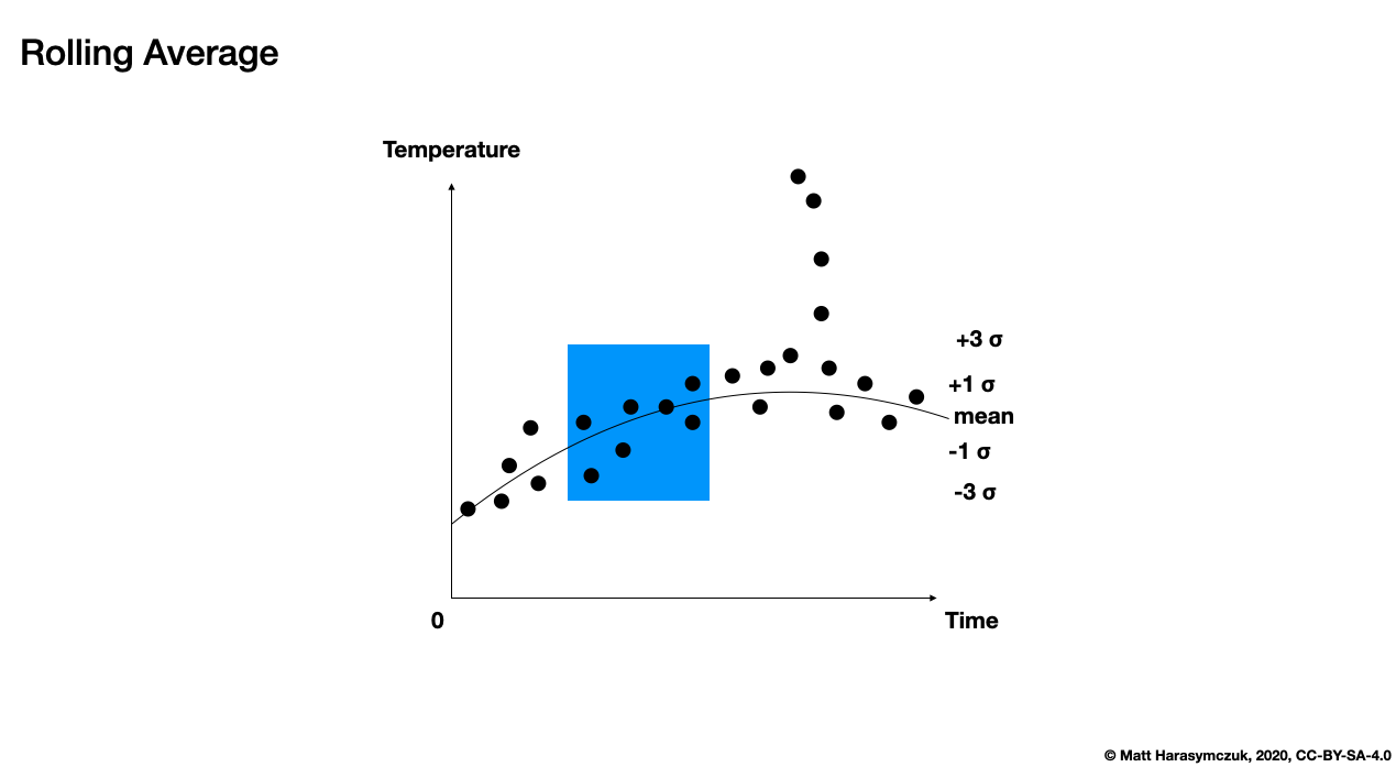
Figure 4.20. Rolling Average

4.11.7. Distribution

Absolute value:

>>> s.abs()
a    1.0
b    2.0
c    3.0
d    NaN
e    5.0
dtype: float64

Standard deviation:

>>> s.std()
1.707825127659933

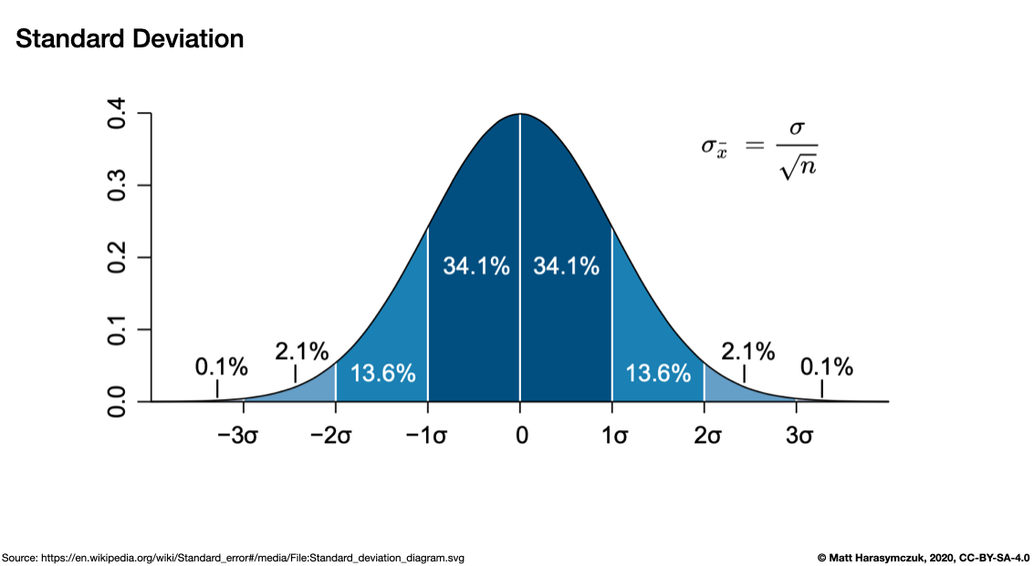
Figure 4.21. Standard Deviation

Standard Error of the Mean (SEM):

>>> s.sem()
0.8539125638299665

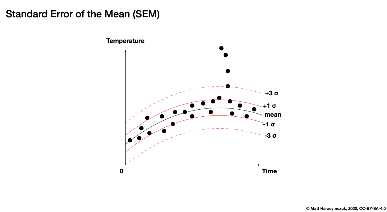
Figure 4.22. Standard Error of the Mean (SEM)

Skewness (3rd moment):

>>> s.skew()
0.7528371991317256

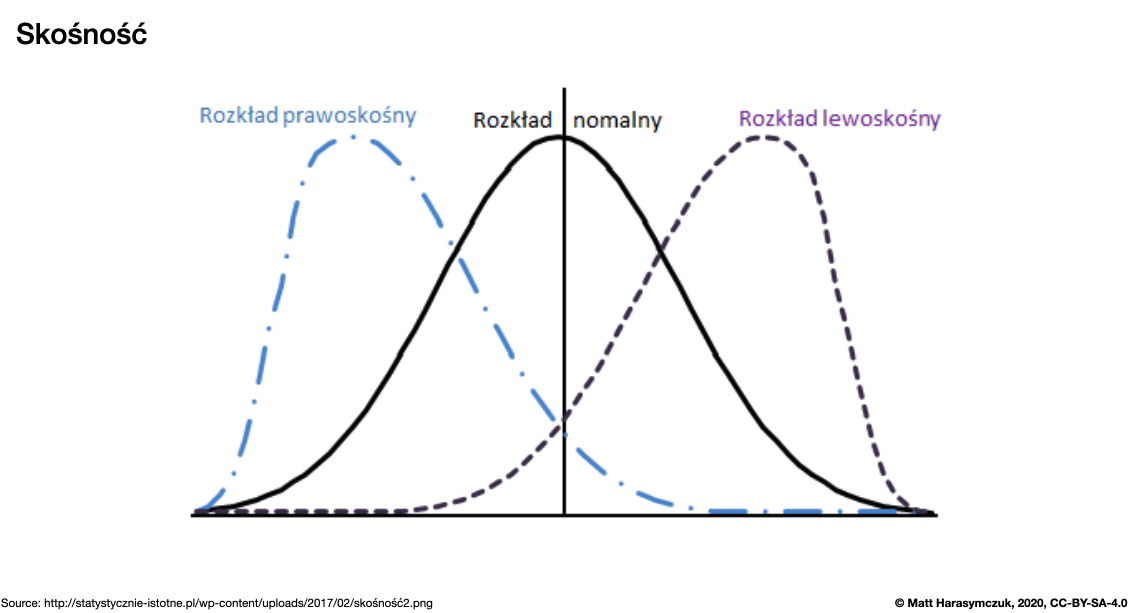
Figure 4.23. Skewness

Kurtosis (4th moment):

>>> s.kurt()
0.3428571428571434

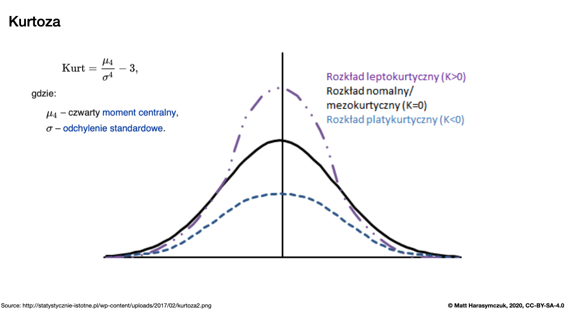
Figure 4.24. Kurtosis

Sample quantile (value at %). Quantile also known as Percentile:

>>> s.quantile(.3)
1.9

>>> s.quantile([.25, .5, .75])
0.25    1.75
0.50    2.50
0.75    3.50
dtype: float64

Variance:

>>> s.var()
2.9166666666666665

Correlation Coefficient:

>>> s.corr(s)
1.0

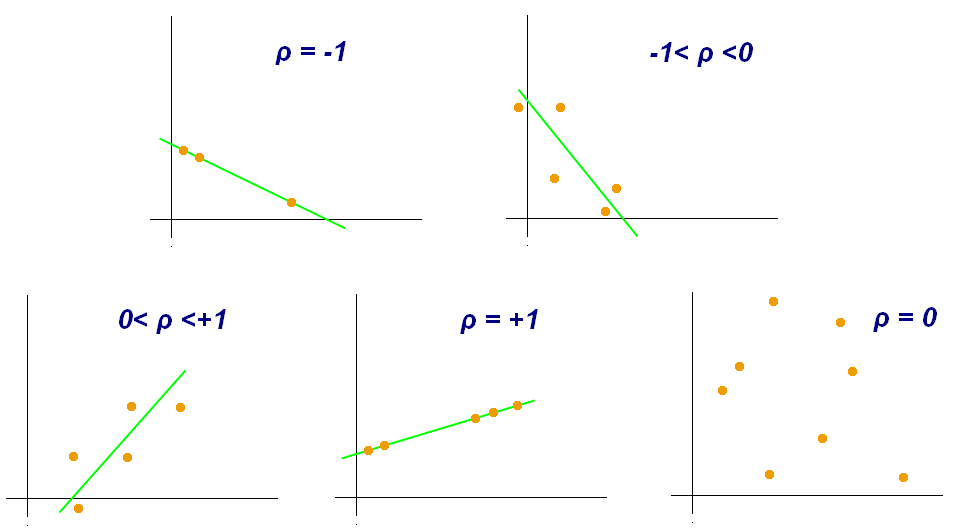
Figure 4.25. Correlation Coefficient

4.11.8. Describe

>>> s.describe()
count    4.000000
mean     2.750000
std      1.707825
min      1.000000
25%      1.750000
50%      2.500000
75%      3.500000
max      5.000000
dtype: float64