5.1. Decision Tree

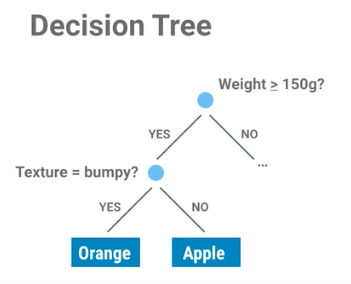
Figure 5.45. Drzewo decyzyjne

from sklearn import tree

# Input to the classifier
# as of Scikit-learn uses real-valued features, we use:
# 0: bumpy
# 1: smooth
#
# features = [
#    [140, 'smooth'],
#    [130, 'smooth'],
#    [150, 'bumpy'],
#    [170, 'bumpy'],
# ]

features = [
    [140, 1],
    [130, 1],
    [150, 0],
    [170, 0],
]

# Output that we want from classifier
# as of Scikit-learn uses real-valued features, we use:
# 0: apple
# 1: orange
#
# labels = ['apple', 'apple', 'orange', 'orange']
labels = [0, 0, 1, 1]


# create decision tree
clf = tree.DecisionTreeClassifier()

# fit - synonim to "find patterns in data"
clf = clf.fit(features, labels)

# use classifier to predict
result = clf.predict([[160, 0]])

print(result)
# should be: [1]

from sklearn import datasets
from sklearn import tree
from sklearn.metrics import accuracy_score
from sklearn.model_selection import train_test_split
from sklearn.neighbors import KNeighborsClassifier

iris = datasets.load_iris()

# Features
x = iris.data

# Labels
y = iris.target

# Split dataset into test and training set in half
x_train, x_test, y_train, y_test = train_test_split(x, y, test_size=0.5)

# Create classifier
decision_tree = tree.DecisionTreeClassifier()

# Train classifier using training data
decision_tree.fit(x_train, y_train)

# Predict
predictions = decision_tree.predict(x_test)

# How accurate was classifier on testing set
# Because of some variation for each run, it might give different results
result = accuracy_score(y_test, predictions)
print(result)
# Output: 0.96

Note identical API for classifiers!

5.1.1. Visualizing a Decision Tree

import numpy
from sklearn.datasets import load_iris
from sklearn import tree

iris = load_iris()

# select test indexes
# dataset is ordered so 0, 50, 100 is a first of each kind
test_idx = [0, 50, 100]


# training data
train_target = numpy.delete(iris.target, test_idx)
train_data = numpy.delete(iris.data, test_idx, axis=0)

# testing data
test_target = iris.target[test_idx]
test_data = iris.data[test_idx]

# create and train classifier
clf = tree.DecisionTreeClassifier()
clf.fit(train_data, train_target)


print(test_target)
# [0 1 2]

result = clf.predict(test_data)
print(result)
# [0 1 2]


print(test_data[0], test_target[0])
# [ 5.1  3.5  1.4  0.2] 0


print(iris.feature_names)
# ['sepal_length (cm)', 'sepal_width (cm)', 'petal_length (cm)', 'petal_width (cm)']

print(iris.target_names)
# ['setosa' 'versicolor' 'virginica']


# Visualization of Decision Tree Classifier
from sklearn.externals.six import StringIO
import pydotplus

dot_data = StringIO()
tree.export_graphviz(
    decision_tree=clf,
    out_file=dot_data,
    feature_names=iris.feature_names,
    class_names=iris.target_names,
    filled=True,
    rounded=True,
    impurity=True
)

graph = pydotplus.graph_from_dot_data(dot_data.getvalue())
graph.write_pdf('/tmp/iris.pdf')

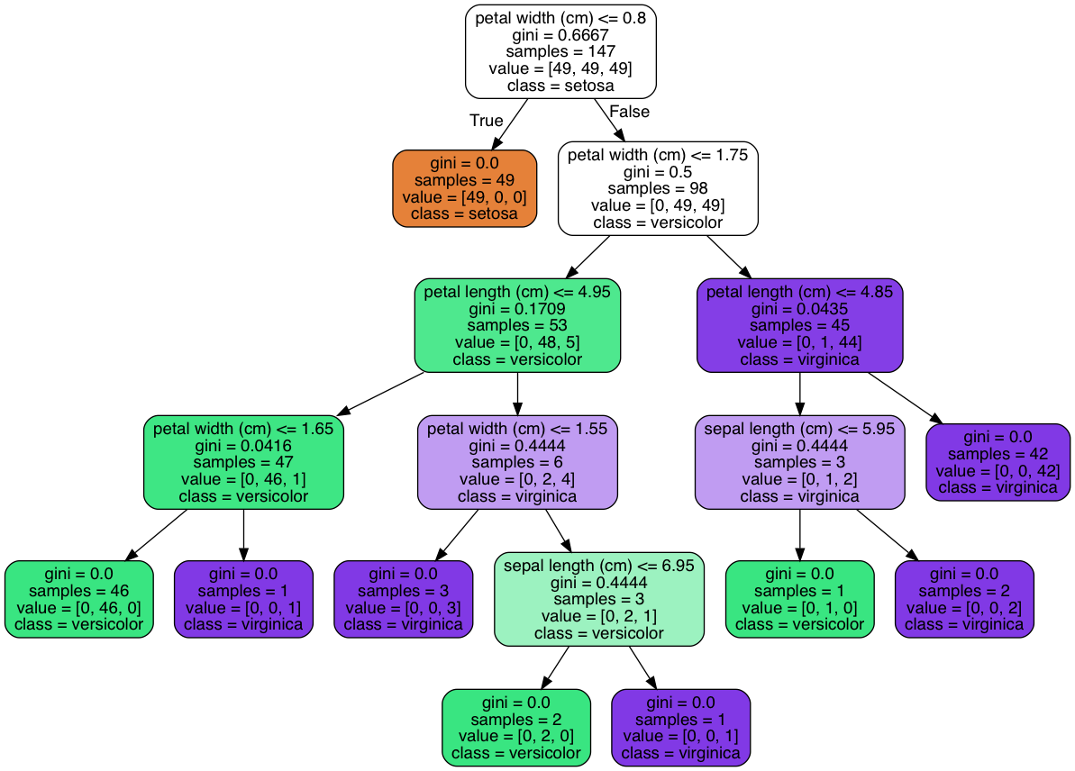
Figure 5.46. Visualization of Decision Tree Classifier

5.1.2. Assignments