6.1. Linear Regression

6.1.1. Co to jest Linear Regression?

The straight line can be seen in the plot, showing how linear regression attempts to draw a straight line that will best minimize the residual sum of squares between the observed responses in the dataset, and the responses predicted by the linear approximation.

The coefficients, the residual sum of squares and the variance score are also calculated.

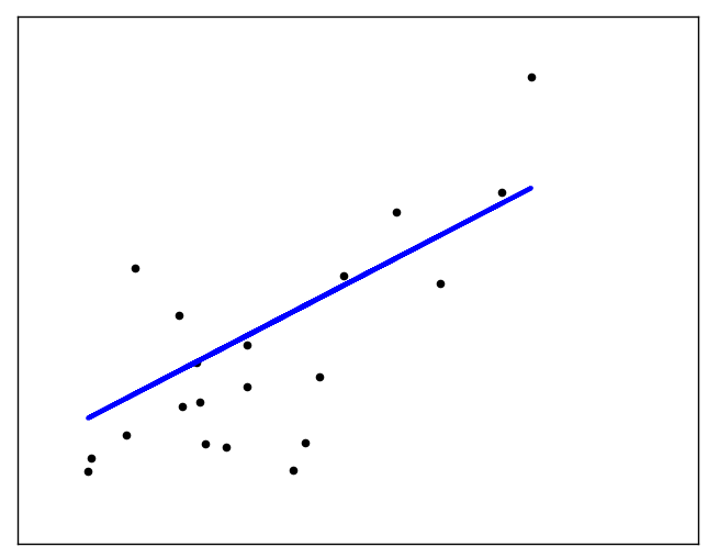
Figure 6.6. The straight line can be seen in the plot, showing how linear regression attempts to draw a straight line that will best minimize the residual sum of squares between the observed responses in the dataset, and the responses predicted by the linear approximation.

6.1.2. Przed zastosowaniem

• Trzeba usunąć elementy odstające

• Trzeba sprawdzić czy są osobne klastry danych, tzn. czy linia jest przedziałami ciągła, tzn. gdyby podzielić na segmenty, to można lepiej dostosować regresję

6.1.3. Wyznaczanie równania prostej

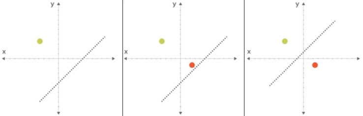
Figure 6.7. Manipulowanie parametrami prostej (klasyfikatora) w celu określenia funkcji.

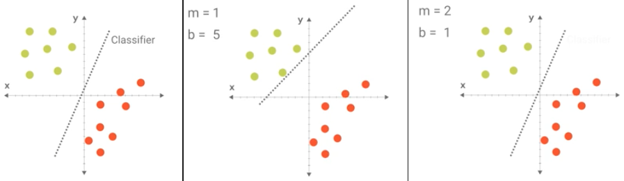
Figure 6.8. Wyznaczanie równania prostej.

6.1.4. Funkcja przedziałami liniowa

Figure 6.9. Funkcja przedziałami liniowa

6.1.5. Przykłady praktyczne

Wykorzystanie biblioteki sklearn

import matplotlib.pyplot as plt
import numpy as np
from sklearn import datasets, linear_model

# Load the diabetes dataset
diabetes = datasets.load_diabetes()

# Use only one feature
diabetes_features = diabetes.data[:, np.newaxis, 2]

# Split the data into training/testing sets
features_train = diabetes_features[:-20]
features_test = diabetes_features[-20:]

# Split the targets into training/testing sets
labels_train = diabetes.target[:-20]
labels_test = diabetes.target[-20:]

# Create linear regression object
model = linear_model.LinearRegression()

# Train the model using the training sets
model.fit(features_train, labels_train)

# The coefficients
print('Coefficients: \n{model.coef_}')

# The mean squared error
print("Mean squared error: %.2f"
      % np.mean((model.predict(features_test) - labels_test) ** 2))

# Explained variance score: 1 is perfect prediction
print('Variance score: %.2f' % model.score(features_test, labels_test))

# Plot outputs
plt.scatter(features_test, labels_test, color='black')
plt.plot(features_test, model.predict(features_test), color='blue', linewidth=3)

plt.xticks(())
plt.yticks(())

plt.show()  # doctest: +SKIP

Coefficients: [ 938.23786125]
Mean squared error: 2548.07
Variance score: 0.4

Figure 6.10. The straight line can be seen in the plot, showing how linear regression attempts to draw a straight line that will best minimize the residual sum of squares between the observed responses in the dataset, and the responses predicted by the linear approximation.

6.1.6. Własna implementacja

import pandas as pd
from math import pow


def cal_mean(readings):
    """
    Function to calculate the mean value of the input readings
    """
    readings_total = sum(readings)
    number_of_readings = len(readings)
    mean = readings_total / float(number_of_readings)
    return mean


def cal_variance(readings):
    """
    Calculating the variance of the readings
    """

    # To calculate the variance we need the mean value
    # Calculating the mean value from the cal_mean function
    readings_mean = cal_mean(readings)

    # mean difference squared readings
    mean_difference_squared_readings = [pow((reading - readings_mean), 2) for reading in readings]
    variance = sum(mean_difference_squared_readings)

    return variance / float(len(readings) - 1)


def cal_covariance(readings_1, readings_2):
    """
    Calculate the covariance between two different list of readings
    """
    readings_1_mean = cal_mean(readings_1)
    readings_2_mean = cal_mean(readings_2)
    readings_size = len(readings_1)
    covariance = 0.0

    for i in range(0, readings_size):
        covariance += (readings_1[i] - readings_1_mean) * (readings_2[i] - readings_2_mean)

    return covariance / float(readings_size - 1)


def cal_simple_linear_regression_coefficients(x_readings, y_readings):
    """
    Calculating the simple linear regression coefficients (B0, B1)
    """

    # Coefficient B1 = covariance of x_readings and y_readings divided by variance of x_readings
    # Directly calling the implemented covariance and the variance functions
    # To calculate the coefficient B1
    b1 = cal_covariance(x_readings, y_readings) / float(cal_variance(x_readings))

    # Coefficient B0 = mean of y_readings - ( B1 * the mean of the x_readings )
    b0 = cal_mean(y_readings) - (b1 * cal_mean(x_readings))

    return b0, b1


def predict_target_value(x, b0, b1):
    """
    Calculating the target (y) value using the input x and the coefficients b0, b1
    """
    return b0 + b1 * x


def cal_rmse(actual_readings, predicted_readings):
    """
    Calculating the root mean square error
    """
    square_error_total = 0.0
    total_readings = len(actual_readings)
    for i in range(0, total_readings):
        error = predicted_readings[i] - actual_readings[i]
        square_error_total += pow(error, 2)
    rmse = square_error_total / float(total_readings)
    return rmse


def simple_linear_regression(dataset):
    """
    Implementing simple linear regression without using any python library
    """

    # Get the dataset header names
    dataset_headers = dataframe.columns.values(dataset)
    print("Dataset Headers :: ", dataset_headers)

    # Calculating the mean of the square feet and the price readings
    square_feet_mean = cal_mean(dataset[dataset_headers[0]])
    price_mean = cal_mean(dataset[dataset_headers[1]])

    square_feet_variance = cal_variance(dataset[dataset_headers[0]])
    price_variance = cal_variance(dataset[dataset_headers[1]])

    # Calculating the regression
    covariance_of_price_and_square_feet = dataset.cov()[dataset_headers[0]][dataset_headers[1]]
    w1 = covariance_of_price_and_square_feet / float(square_feet_variance)

    w0 = price_mean - (w1 * square_feet_mean)

    # Predictions
    dataset['Predicted_Price'] = w0 + w1 * dataset[dataset_headers[0]]


if __name__ == "__main__":
    input_path = '../_data/input-data.csv'
    house_price_dataset = pd.read_csv(input_path)
    simple_linear_regression(house_price_dataset)

6.1.7. Assignments

6.1.7.1. Least square regression 3 points

• Assignment: Least square regression 3 points

• Complexity: easy

• Lines of code: 10 lines

• Time: 13 min

English:

1. Consider the following set of points: \({(-2 , -1) , (1 , 1) , (3 , 2)}\)

2. Find the least square regression line for the given data points.

3. Plot the given points and the regression line in the same rectangular system of axes.

4. Napisz własny kod implementujący rozwiązanie

5. Run doctests - all must succeed

Polish:

6.1.7.2. Least square regression 4 points

• Assignment: Least square regression 4 points

• Complexity: easy

• Lines of code: 10 lines

• Time: 13 min

English:

1. Find the least square regression line for the following set of data: \({(-1 , 0),(0 , 2),(1 , 4),(2 , 5)}\)

2. Plot the given points and the regression line in the same rectangular system of axes.

3. Użyj kodu z przykładu własnej implementacji do rozwiązania

4. Run doctests - all must succeed

Polish:

6.1.7.3. Company sales

• Assignment: Company sales

• Complexity: easy

• Lines of code: 10 lines

• Time: 13 min

English:

1. The sales of a company (in million dollars) for each year are shown in the table below.

   x (year)    2005    2006    2007    2008    2009
   y (sales)   12      19      29      37      45
   

2. Find the least square regression line \(y = ax + b\) .

3. Use the least squares regression line as a model to estimate the sales of the company in 2012.

4. Use sklearn

5. Run doctests - all must succeed

Polish: