4.2. Principal Component Analysis

• Principal component analysis (PCA)

• Technique used to emphasize variation and bring out strong patterns in a dataset.

• It's often used to make data easy to explore and visualize.

• Linear dimensionality reduction using Singular Value Decomposition of the data to project it to a lower dimensional space.

4.2.1. What is Principal Component Analysis?

4.2.2. 2D example

• http://setosa.io/ev/principal-component-analysis/

First, consider a dataset in only two dimensions, like (height, weight). This dataset can be plotted as points in a plane. But if we want to tease out variation, PCA finds a new coordinate system in which every point has a new (x,y) value. The axes don't actually mean anything physical; they're combinations of height and weight called "principal components" that are chosen to give one axes lots of variation.

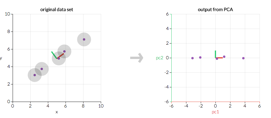
Figure 4.73. PCA is useful for eliminating dimensions. If we're going to only see the data along one dimension, though, it might be better to make that dimension the principal component with most variation. We don't lose much by dropping PC2 since it contributes the least to the variation in the data set.

import numpy as np
from sklearn.decomposition import PCA

X = np.array([[-1, -1], [-2, -1], [-3, -2], [1, 1], [2, 1], [3, 2]])

pca = PCA(n_components=2)
pca.fit(X)
# PCA(copy=True, iterated_power='auto', n_components=2, random_state=None,
#     svd_solver='auto', tol=0.0, whiten=False)

pca.explained_variance_ratio_
# [ 0.99244...  0.00755...]

pca = PCA(n_components=2, svd_solver='full')

pca.fit(X)
# PCA(copy=True, iterated_power='auto', n_components=2, random_state=None,
#     svd_solver='full', tol=0.0, whiten=False)

pca.explained_variance_ratio_
# [ 0.99244...  0.00755...]

pca = PCA(n_components=1, svd_solver='arpack')

pca.fit(X)
# PCA(copy=True, iterated_power='auto', n_components=1, random_state=None,
#     svd_solver='arpack', tol=0.0, whiten=False)

pca.explained_variance_ratio_
# [ 0.99244...]

4.2.3. 3D example

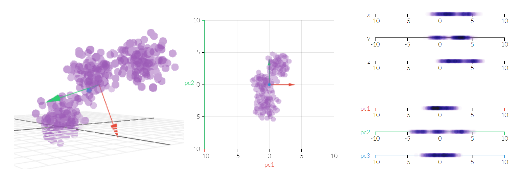
Figure 4.74. Principal Component Analysis 3D

4.2.4. Przykłady praktyczne

• https://github.com/scikit-learn/scikit-learn/tree/master/examples/decomposition

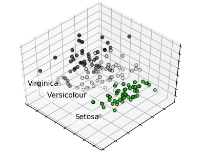
4.2.5. PCA dla zbioru Iris

import numpy as np
import matplotlib.pyplot as plt
from mpl_toolkits.mplot3d import Axes3D
from sklearn import decomposition
from sklearn import datasets


iris = datasets.load_iris()
features = iris.data
labels = iris.target

pca = decomposition.PCA(n_components=3)
pca.fit(features)
features = pca.transform(features)

plt.clf()  # doctest: +SKIP

fig = plt.figure(1, figsize=(4, 3))
ax = Axes3D(fig, rect=[0, 0, .95, 1], elev=48, azim=134)

plt.cla()  # doctest: +SKIP


for name, label in [('Setosa', 0), ('Versicolor', 1), ('Virginica', 2)]:
    ax.text3D(
        features[labels == label, 0].mean(),
        features[labels == label, 1].mean() + 1.5,
        features[labels == label, 2].mean(), name,
        horizontalalignment='center',
        bbox=dict(alpha=0.5, edgecolor='w', facecolor='w'))

# Reorder the labels to have colors matching the cluster results
labels = np.choose(labels, [1, 2, 0]).astype(np.float)
ax.scatter(features[:, 0], features[:, 1], features[:, 2], c=labels, edgecolor='k')

ax.w_xaxis.set_ticklabels([])
ax.w_yaxis.set_ticklabels([])
ax.w_zaxis.set_ticklabels([])

plt.show()  # doctest: +SKIP

PCA dla zbioru Iris:

4.2.6. Assignments

4.2.6.1. PCA dla zbioru Pima Indian Diabetes

• Assignment: PCA dla zbioru Pima Indian Diabetes

• Complexity: medium

• Lines of code: 30 lines

• Time: 21 min

English:

TODO: English Translation X. Run doctests - all must succeed

Polish:

1. Przeprowadź analizę PCA dla zbioru Indian Pima

2. Uruchom doctesty - wszystkie muszą się powieść