4.1. Model Quality

4.1.1. Metody doboru modelu i poprawienia jakości

• Walidacje

• Poszukiwanie parametrów

• Regularyzacja

• Ensemble

4.1.2. Słownictwo

Cost Function

A cost function is something you want to minimize. For example, your cost function might be the sum of squared errors over your training set. Gradient descent is a method for finding the minimum of a function of multiple variables.

Loss function

is used to measure the degree of fit. So for machine learning a few elements are:

• Hypothesis space: e.g. parametric form of the function such as linear regression, logistic regression, svm, etc.

• Measure of fit: loss function, likelihood

• Tradeoff between bias vs. variance: regularization. Or bayesian estimator (MAP)

• Find a good h in hypothesis space: optimization. convex - global. non-convex - multiple starts

• Verification of h: predict on test data. cross validation.

4.1.3. Diagnostyka Bias vs. Wariancja

Osiąganie kiepskich rezultatów na zbiorze testowym wiąże się zazwyczaj z jednym z dwóch zjawisk:

• wysoki bias - niedopasowanie (under fitting)

• wysoka wariancja - nadmierne dopasowanie (over fitting)

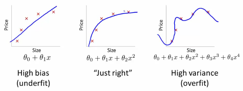
Figure 4.66. Bias vs. Wariancja

Ważne, żebyśmy zorientowali się, co jest naszym problemem. Mamy możliwe trzy sytuacje: wysoki bias, wysoką wariancję, bądź wreszcie dobre dopasowanie. Graficznie wygląda to tak:

Jak można powyżej zauważyć, stopień wielomianu (który dopasowujemy do danych) rośnie, gdy przesuwamy się w stronę overfittingu.

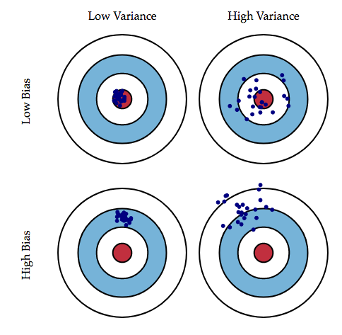
Figure 4.67. Graphical illustration of bias and variance.

4.1.4. Decydowanie o kolejnym kroku

Jakich zmian dokonać w naszym algorytmie, jeżeli błędy są za duże? Możliwe rozwiązania to:

• Stworzyć więcej przypadków testowych (pomaga przy nadmiernym dopasowaniu)

• Zmniejszyć zbiór wykorzystywanych cech (pomaga przy nadmiernym dopasowaniu)

• Wykorzystać dodatkowe cechy (pomaga przy słabym dopasowaniu)

• Dodać cechy wielomianowe (pomaga przy słabym dopasowaniu)

• Zmniejszyć lambdę (pomaga przy słabym dopasowaniu)

• Zwiększyć lambdę (pomaga przy nadmiernym dopasowaniu)

4.1.5. Overfitting w sieciach neuronowych

Tworząc sieci neuronowe mamy dwie opcje:

• Możemy wykorzystać mniejszą sieć z niewielką liczbą ukrytych warstw i ukrytych jednostek. Jest ona bardziej podatna na underfitting. Jej główną zaletą jest niewielka złożoność obliczeniowa.

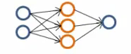
Figure 4.68. Prosta jednowarstwowa sieć neuronowa.

• Możemy wykorzystać relatywnie dużą sieć neuronową, która zawiera więcej ukrytych jednostek lub więcej ukrytych warstw. Jest bardziej podatna na overfitting oraz ma większą złożoność.

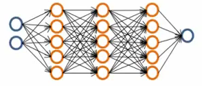
Figure 4.69. Głęboka sieć neuronowa.

• Najczęściej wykorzystanie dużej sieci neuronowej z regularyzacją (w celu zmniejszenia overfittingu) jest bardziej efektywne od stworzenia małej sieci. Decyzję o liczbie ukrytych warstw można podjąć mierząc błąd zbioru testowego dla różnych wariantów i wybierając liczbę warstw przy której błąd ten jest najmniejszy.

4.1.6. Model Evaluation Procedure

4.1.7. Train and test on entire dataset

1. Train the model on entire dataset

2. Test the model on the same dataset, and evaluate how well we did by comparing the predicted response value with the true response values.

from sklearn.datasets import load_iris

iris = load_iris()

features = iris.data
labels = iris.target

1. Classification accuracy

   • Proportion of correct predictions

   • Common evaluation metric for classification problems

   • Known as training accuracy when you train and test the model on the same data

2. Problems with training and testing on the same data

   • Goal is to estimate likely performance of a model on out-of-sample data

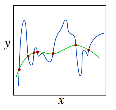
   • But, maximizing training accuracy rewards overly complex models that won't necessarily generalize

   • Unnecessarily complex models overfit the data

   • Models that overfit learns to recognize noise from the signal, than the data

   • KNeighborsClassifier(n_neighbors=1) memorizes training data and uses test data to check the same places

   • Very low \(k\) values creates complicated overfit model

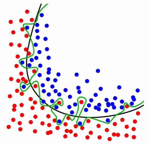
Figure 4.70. Models that overfit learns to recognize noise from the signal, than the data. Black line represents the decision boundary and represents the signal. Green line represents overfitted model which learned the noise.

Testing LogisticsRegression on Iris dataset:

from sklearn.linear_model import LogisticsRegression
from sklearn import metrics

model = LogisticsRegression()
model.fit(features, labels)
predicted_labels = model.predict(features)

metrics.accuracy_score(labels, predicted_labels)
# 0.96

Testing KNeighborsClassifier(n_neighbors=1) on Iris dataset:

from sklearn.neighbors import KNeighborsClassifier
from sklearn import metrics

model = KNeighborsClassifier(n_neighbors=1)
model.fit(features, labels)
predicted_labels = model.predict(features)

metrics.accuracy_score(labels, predicted_labels)
# 1.0

Testing KNeighborsClassifier(n_neighbors=5) on Iris dataset:

from sklearn.neighbors import KNeighborsClassifier
from sklearn import metrics

model = KNeighborsClassifier(n_neighbors=5)
model.fit(features, labels)
predicted_labels = model.predict(features)

accuracy = metrics.accuracy_score(labels, predicted_labels)
# 0.966666666667

4.1.8. Train/test split

Also known as:

• Test set approach

• Validation set approach

1. Split the dataset into two pieces:

   • a training set

   • a testing set

2. Train the model on a training set.

3. Test the model on a testing set, and evaluate how well we did.

from sklearn.model_selection import train_test_split

# Split the data into training and testing sets
features_train, features_test, labels_train, labels_test = train_test_split(features, labels, test_size=0.4)

1. If you do not use optional integer parameter random_state to train_test_split it will randomize splitting data

2. Models can be trained and tested on different data

3. Response values are known for the training set, and thus predictions can be evaluated

4. Testing accuracy is a better estimate than training accuracy of out-of-sample performance

Testing LogisticsRegression on Iris dataset:

from sklearn.linear_model import LogisticsRegression
from sklearn import metrics

model = LogisticsRegression()
model.fit(features_train, labels_train)
predicted_labels = model.predict(features_test)

accuracy = metrics.accuracy_score(labels_test, predicted_labels)
# 0.95

Testing KNeighborsClassifier(n_neighbors=1) on Iris dataset:

from sklearn.neighbors import KNeighborsClassifier
from sklearn import metrics

model = KNeighborsClassifier(n_neighbors=1)
model.fit(features_train, labels_train)
predicted_labels = model.predict(features_test)

accuracy = metrics.accuracy_score(labels_test, predicted_labels)
# 0.95

Testing KNeighborsClassifier(n_neighbors=5) on Iris dataset:

from sklearn.neighbors import KNeighborsClassifier
from sklearn import metrics

model = KNeighborsClassifier(n_neighbors=5)
model.fit(features_train, labels_train)
predicted_labels = model.predict(features_test)

accuracy = metrics.accuracy_score(labels_test, predicted_labels)
# 0.966666666667

Can we locate even better value for \(k\)?:

1. Testing accuracy raises as model complexity increases

2. Testing accuracy penalizes models that are too complex or not complex enough

3. For KNN models complexity is determined by the value of \(k\) (lower value = more complex)

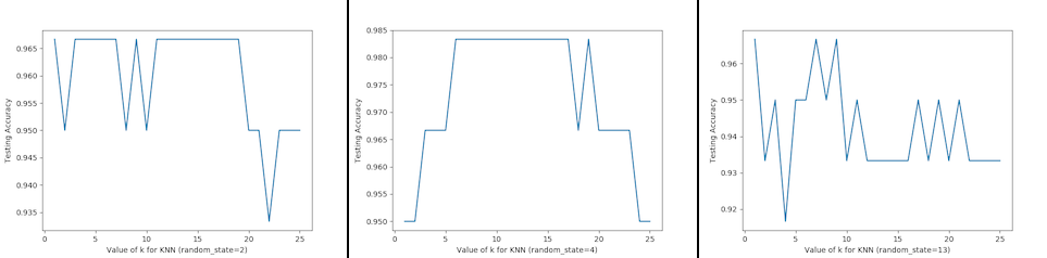
Figure 4.71. For KNN models complexity is determined by the value of \(k\) (lower value = more complex)

from sklearn.neighbors import KNeighborsClassifier
from sklearn import metrics
from sklearn.datasets import load_iris
from sklearn.model_selection import train_test_split
import matplotlib.pyplot as plt

iris = load_iris()
features = iris.data
labels = iris.target

random_state = 4
k_range = range(1, 26)
scores = []

features_train, features_test, labels_train, labels_test = train_test_split(
    features, labels, random_state=random_state, test_size=0.4)

for k in k_range:
    model = KNeighborsClassifier(n_neighbors=k)
    model.fit(features_train, labels_train)
    predicted_labels = model.predict(features_test)

    accuracy = metrics.accuracy_score(labels_test, predicted_labels)
    scores.append(accuracy)

plt.plot(k_range, scores)
plt.xlabel(f'Value of k for KNN (random_state={random_state})')
plt.ylabel('Testing Accuracy')
plt.show()  # doctest: +SKIP

Downsides of train/test split:

1. Provides a high-variance estimate of out-of-sample accuracy

2. \(K\) - fold cross-validation overcomes the limitation

3. Train/test split is still used because of its flexibility and speed

Source: https://www.dataschool.io

4.1.9. Regularyzacja

• Regularyzacja – wprowadzenie dodatkowej informacji do rozwiązywanego zagadnienia źle postawionego w celu polepszenia jakości rozwiązania.

• Regularyzacja jest często wykorzystywana przy rozwiązywaniu problemów odwrotnych.

• Regularyzacja jest sposobem na zmniejszenie prawdopodobieństwa pojawienia się overfittingu

4.1.10. Random Forrest

A random forest is a meta estimator that fits a number of decision tree classifiers on various sub-samples of the dataset and use averaging to improve the predictive accuracy and control over-fitting. The sub-sample size is always the same as the original input sample size but the samples are drawn with replacement if bootstrap=True (default).

4.1.11. Ensemble averaging

• In machine learning, particularly in the creation of artificial neural networks, ensemble averaging is the process of creating multiple models and combining them to produce a desired output, as opposed to creating just one model.

• Frequently an ensemble of models performs better than any individual model, because the various errors of the models "average out."

• Ensemble averaging is one of the simplest types of committee machines. Along with boosting, it is one of the two major types of static committee machines.

• In contrast to standard network design in which many networks are generated but only one is kept, ensemble averaging keeps the less satisfactory networks around, but with less weight.

• The theory of ensemble averaging relies on two properties of artificial neural networks:

  1. In any network, the bias can be reduced at the cost of increased variance

  2. In a group of networks, the variance can be reduced at no cost to bias

• In machine learning ensemble refers only to a concrete finite set of alternative models, but typically allows for much more flexible structure to exist among those alternatives.

import numpy as np
from sklearn import preprocessing
from sklearn.ensemble import ExtraTreesClassifier


with open('../_data/pima-diabetes.csv') as file:
    dataset = np.loadtxt(file, delimiter=",")
    features = dataset[:, :-1]
    labels = dataset[:, -1]


# Normalize and Standardize the features so that it does not affect the learning algorithm
preprocessing.normalize(features)
preprocessing.scale(features)

# Fit the Tree algorithm
model = ExtraTreesClassifier()
model.fit(features, labels)

# display the relative importance of each attribute
print(model.feature_importances_)

4.1.12. Benefits

• The resulting committee is almost always less complex than a single network which would achieve the same level of performance

• The resulting committee can be trained more easily on smaller input sets

• The resulting committee often has improved performance over any single network

• The risk of overfitting is lessened, as there are fewer parameters (weights) which need to be set