11.1. Deep Neural Network

11.1.1. What Is a Neural Network?

It's a technique for building a computer program that learns from data. It is based very loosely on how we think the human brain works. First, a collection of software "neurons" are created and connected together, allowing them to send messages to each other. Next, the network is asked to solve a problem, which it attempts to do over and over, each time strengthening the connections that lead to success and diminishing those that lead to failure. For a more detailed introduction to neural networks, Michael Nielsen's Neural Networks and Deep Learning is a good place to start. For a more technical overview, try Deep Learning by Ian Goodfellow, Joshua Bengio, and Aaron Courville.

Neural Networks are the best Machine Learning algorithm so far.

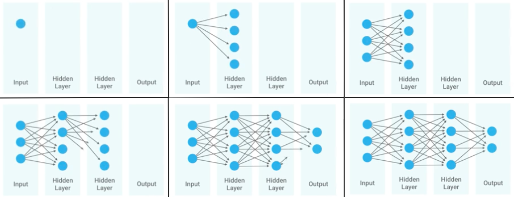
../../_images/deep-neural-network.png — Figure 11.1. Neural Network

11.1.2. Słownictwo

overfitting: gdy sieć neuronowa jest tak dobrze nauczona, że dane które przychodzą mają problem z byciem dobrze sklasyfikowanymi
shallow learning: Gdy wartość output zależy od jednego poziomu parametrów. Sumujemy wagi i wartości i dostajemy liczbę na końcu. Można wykreślić prostą funkcję liniową lub kwadratową. Należy zwrócić uwagę aby nie doprowadzić do overfitting.
deep Learning: Wartość zależy od kilku poziomów sieci.
back propagation: zmiana wartości wag w sieci neuronowej na niższych warstwach - propagacja w dół sieci
neuron
weight
input Layer
hidden Layer
output Layer
fully connected layer
activation function

11.1.3. Przykład praktyczny

Wyobraźmy sobie ofertę domu.
Każdy z elementów oferty ma swoje atrybuty:
- basen
- ilość sypialni
- rok budowy
- ogród
- domek dla gości
- garaż
- lokacja
- powierzchnia
- wyposażenie
Wpływa na cenę domu w różnym stopniu
Niektóre rzeczy mają większą wagę, tzn. lokacja mocno podnosi cenę, a garaż zdecydowanie mniej
Wewnątrz sieci, neurony składają się z pewnych liniowych lub nieliniowych zależności pomiędzy poszczególnymi atrybutami oferty
Przykład poziomu hidden layer:
- mały dom w dobrej lokalizacji
- duży dom w gorszej lokalizacji
- umiarkowana lokalizacja i rozmiar plus basen
Cena domu wpływa na sumę wszystkich kombinacji elementów i ich wag z poprzednich stopni.

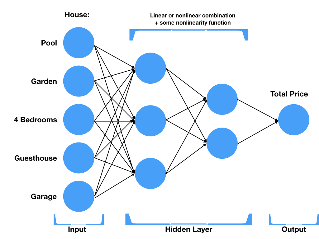
../../_images/neural-network.png — Figure 11.2. Neural Network

11.1.4. Tools

TensorFlow (Google) - http://playground.tensorflow.org/

11.1.5. Inception

One of Google's best image classifiers
Open Source
Trained on 1.2 milion images
Training took 2 weeks on 8GPU machine

11.1.6. Działanie na sieciach neuronowych

11.1.7. Construction

Ilość neuronów
Poziom zagłębień

11.1.8. Learning

11.1.9. Optimizing

11.1.10. Retraining

Also known as Transfer Learning
Saves a lot of time
Uses prior work

11.1.11. Przetwarzanie obrazów na przykładzie rozpoznawania odręcznie napisanych cyfr (MNIST)

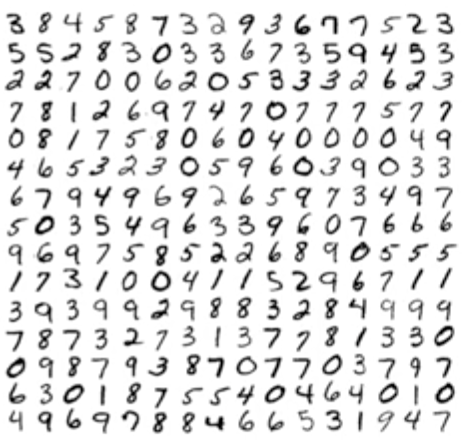
../../_images/deep-neural-networks-mnist-overview.png — Figure 11.3. Handwritten digits recognition also known as MNIST is equivalent to "hello world" in visual Machine Learning world.

11.1.12. Flattening image

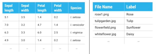
../../_images/dnn-images.png — Figure 11.4. In Image processing files and image pixels are features.

Używanie "raw pixels" as features
Classifier does the rest

Flatten image: 2D array -> 1D by unstacking rows and lining them up (reshape array):

import matplotlib.pyplot as plt

def display(i):
    img = test_data[i]
    plt.title('Example %d. Label: %d' % (i, test_labels[i]))
    plt.imshow(img.reshape((28,28)), cmap=plt.cm.gray_r)

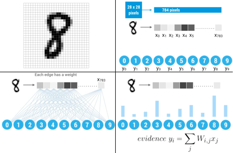
../../_images/deep-neural-networks-mnist-segmented.png — Figure 11.5. Segmented Digit

11.1.13. Weight adjusted by gradient descent

Begin with random weight
Gradually adjust to better values
Evaluate accuracy

../../_images/deep-neural-networks-mnist-pixels.png — Figure 11.6. Compare middle image pixel.

11.1.14. Visualize weights

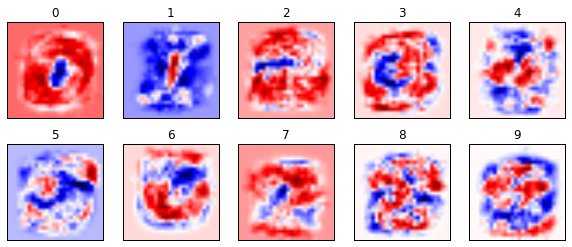
../../_images/deep-neural-networks-mnist-weights.png — Figure 11.7. Visualize the the weights in the TensorFlow Basic MNIST

11.1.15. Przykłady praktyczne

11.1.16. Image Classification using `TensorFlow for Poets`

https://codelabs.developers.google.com/codelabs/tensorflow-for-poets/#1

download around 218MB of data:

$ curl -O http://download.tensorflow.org/example_images/flower_photos.tgz
$ tar xzf flower_photos.tgz
$ ls flower_photos

Training on this much data can take 30+ minutes on a small computer. If you want to reduce data:

$ ls flower_photos/roses | wc -l
$ rm flower_photos/*/[3-9]*
$ ls flower_photos/roses | wc -l

from sklearn import metrics
from sklearn import model_selection
import tensorflow as tf
from tensorflow.contrib import learn


# Load dataset
iris = learn.datasets.load_dataset('iris')
x_train, x_test, y_train, y_test = model_selection.train_test_split(
    iris.data,
    iris.target,
    test_size=0.2,
    random_state=42
)

# Build 3 layer Deep Neural Network (DNN) with 10, 20, 10 units respectively.
classifier = learn.DNNClassifier(hidden_units=[10, 20, 10], n_classes=3)

# Fit and predict.
classifier.fit(x_train, y_train, steps=200)
score = metrics.accuracy_score(y_test, classifier.predict(x_test))

print(f'Accuracy {score:f}')

$ curl -O https://raw.githubusercontent.com/tensorflow/tensorflow/r1.1/tensorflow/examples/image_retraining/retrain.py

$ python retrain.py \
  --bottleneck_dir=bottlenecks \
  --how_many_training_steps=500 \
  --model_dir=inception \
  --summaries_dir=training_summaries/basic \
  --output_graph=retrained_graph.pb \
  --output_labels=retrained_labels.txt \
  --image_dir=flower_photos

[...]
2017-07-01 11:10:43.635017: Step 499: Train accuracy = 88.0%
2017-07-01 11:10:43.635265: Step 499: Cross entropy = 0.455413
2017-07-01 11:10:44.201455: Step 499: Validation accuracy = 92.0% (N=100)

Final test accuracy = 87.3% (N=331)

$ curl -L https://goo.gl/3lTKZs > label_image.py

$ python label_image.py flower_photos/daisy/21652746_cc379e0eea_m.jpg
daisy (score = 0.98659)
sunflowers (score = 0.01068)
dandelion (score = 0.00204)
tulips (score = 0.00063)
roses (score = 0.00007)

$ python label_image.py flower_photos/roses/2414954629_3708a1a04d.jpg
roses (score = 0.84563)
tulips (score = 0.13727)
dandelion (score = 0.00897)
sunflowers (score = 0.00644)
daisy (score = 0.00169)

11.1.17. Face completion with a multi-output estimators

This example shows the use of multi-output estimator to complete images. The goal is to predict the lower half of a face given its upper half.

The first column of images shows true faces. The next columns illustrate how extremely randomized trees, k nearest neighbors, linear regression and ridge regression complete the lower half of those faces.

import numpy as np
import matplotlib.pyplot as plt

from sklearn.datasets import fetch_olivetti_faces
from sklearn.utils.validation import check_random_state

from sklearn.ensemble import ExtraTreesRegressor
from sklearn.neighbors import KNeighborsRegressor
from sklearn.linear_model import LinearRegression
from sklearn.linear_model import RidgeCV

# Load the faces datasets
data = fetch_olivetti_faces()
targets = data.target

data = data.images.reshape((len(data.images), -1))
train = data[targets < 30]
test = data[targets >= 30]  # Test on independent people

# Test on a subset of people
n_faces = 5
rng = check_random_state(4)
face_ids = rng.randint(test.shape[0], size=(n_faces, ))
test = test[face_ids, :]

n_pixels = data.shape[1]
# Upper half of the faces
X_train = train[:, :(n_pixels + 1) // 2]
# Lower half of the faces
y_train = train[:, n_pixels // 2:]
X_test = test[:, :(n_pixels + 1) // 2]
y_test = test[:, n_pixels // 2:]

# Fit estimators
ESTIMATORS = {
    "Extra trees": ExtraTreesRegressor(n_estimators=10, max_features=32,
                                       random_state=0),
    "K-nn": KNeighborsRegressor(),
    "Linear regression": LinearRegression(),
    "Ridge": RidgeCV(),
}

y_test_predict = dict()
for name, estimator in ESTIMATORS.items():
    estimator.fit(X_train, y_train)
    y_test_predict[name] = estimator.predict(X_test)

# Plot the completed faces
image_shape = (64, 64)

n_cols = 1 + len(ESTIMATORS)
plt.figure(figsize=(2. * n_cols, 2.26 * n_faces))
plt.suptitle("Face completion with multi-output estimators", size=16)

for i in range(n_faces):
    true_face = np.hstack((X_test[i], y_test[i]))

    if i:
        sub = plt.subplot(n_faces, n_cols, i * n_cols + 1)
    else:
        sub = plt.subplot(n_faces, n_cols, i * n_cols + 1,
                          title="true faces")

    sub.axis("off")
    sub.imshow(true_face.reshape(image_shape),
               cmap=plt.cm.gray,
               interpolation="nearest")

    for j, est in enumerate(sorted(ESTIMATORS)):
        completed_face = np.hstack((X_test[i], y_test_predict[est][i]))

        if i:
            sub = plt.subplot(n_faces, n_cols, i * n_cols + 2 + j)

        else:
            sub = plt.subplot(n_faces, n_cols, i * n_cols + 2 + j,
                              title=est)

        sub.axis("off")
        sub.imshow(completed_face.reshape(image_shape),
                   cmap=plt.cm.gray,
                   interpolation="nearest")

plt.show()  # doctest: +SKIP

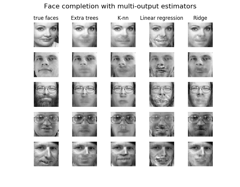
../../_images/visual-faces.png — Figure 11.8. This example shows the use of multi-output estimator to complete images. The goal is to predict the lower half of a face given its upper half.