10.1. K-Means Clustering

A loose definition of clustering could be "the process of organizing objects into groups whose members are similar in some way". A cluster is therefore a collection of objects which are "similar" between them and are "dissimilar" to the objects belonging to other clusters.

• Clustering algorithms are usually unsupervised.

• How many groups (clusters) you want your data to be in?

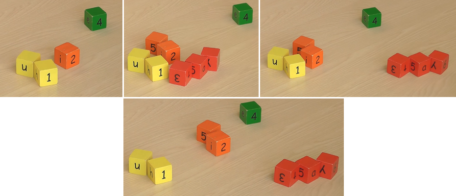
Figure 10.5. Clustering (grouping) data.

• When you sort data in unsupervised learning you quite often ends up with looking good at the beginning.

• When you look at data from different perspective it's not so great.

• Algorithms only work when you tell them, how many groups you want data in.

10.1.1. Przykłady zastosowania

• pixels colors

• patients in hospital: how sick they are

• cars: new, used

• jobs: different kinds

10.1.2. Algorytmy klastrowania

Method name	Parameters	Scalability	Usecase	Geometry (metric used)
K-Means	number of clusters	Very large n_samples, medium n_clusters with MiniBatch code	General-purpose, even cluster size, flat geometry, not too many clusters	Distances between points
Affinity propagation	damping, sample preference	Not scalable with n_samples	Many clusters, uneven cluster size, non-flat geometry	Graph distance (e.g. nearest-neighbor graph)
Mean-shift	bandwidth	Not scalable with n_samples	Many clusters, uneven cluster size, non-flat geometry	Distances between points
Spectral clustering	number of clusters	Medium n_samples, small n_clusters	Few clusters, even cluster size, non-flat geometry	Graph distance (e.g. nearest-neighbor graph)
Ward hierarchical clustering	number of clusters	Large n_samples and n_clusters	Many clusters, possibly connectivity constraints	Distances between points
Agglomerative clustering	number of clusters, linkage type, distance	Large n_samples and n_clusters	Many clusters, possibly connectivity constraints, non Euclidean distances	Any pairwise distance
DBSCAN	neighborhood size	Very large n_samples, medium n_clusters	Non-flat geometry, uneven cluster sizes	Distances between nearest points
Gaussian mixtures	many	Not scalable	Flat geometry, good for density estimation	Mahalanobis distances to centers
Birch	branching factor, threshold, optional global clusterer.	Large n_clusters and n_samples	Large dataset, outlier removal, data reduction.	Euclidean distance between points

10.1.3. Similarities

• statistical

• algebraical

• geometrical

10.1.4. Flat Clustering

Clustering algorithms group a set of documents into subsets or clusters . The algorithms' goal is to create clusters that are coherent internally, but clearly different from each other. In other words, documents within a cluster should be as similar as possible; and documents in one cluster should be as dissimilar as possible from documents in other clusters.

10.1.5. K-means

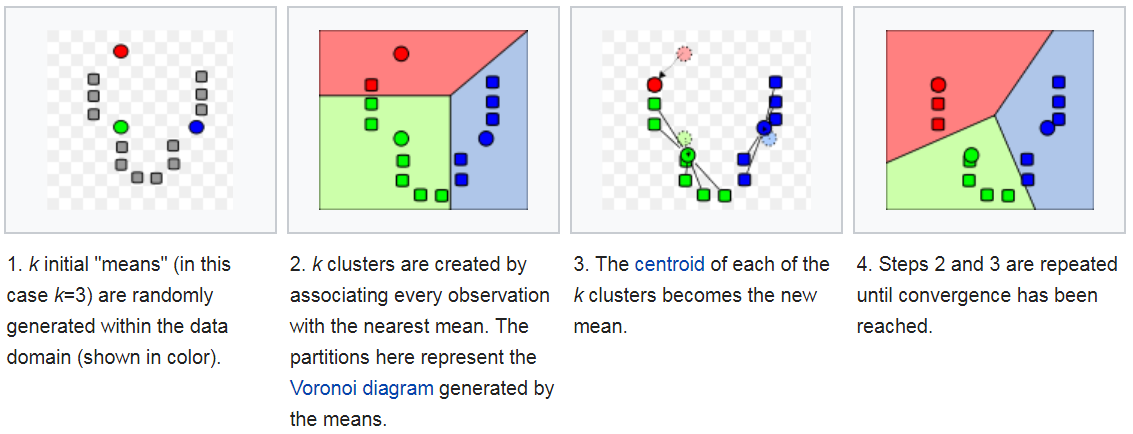
K-means Convergence:

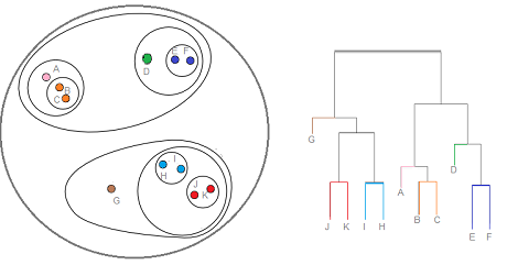
10.1.6. Hierarchical Clustering

Hierarchical clustering is where you build a cluster tree (a dendrogram) to represent data, where each group (or "node") is linked to two or more successor groups. The groups are nested and organized as a tree, which ideally ends up as a meaningful classification scheme.

Each node in the cluster tree contains a group of similar data; Nodes are placed on the graph next to other, similar nodes. Clusters at one level are joined with clusters in the next level up, using a degree of similarity; The process carries on until all nodes are in the tree, which gives a visual snapshot of the data contained in the whole set. The total number of clusters is not predetermined before you start the tree creation.

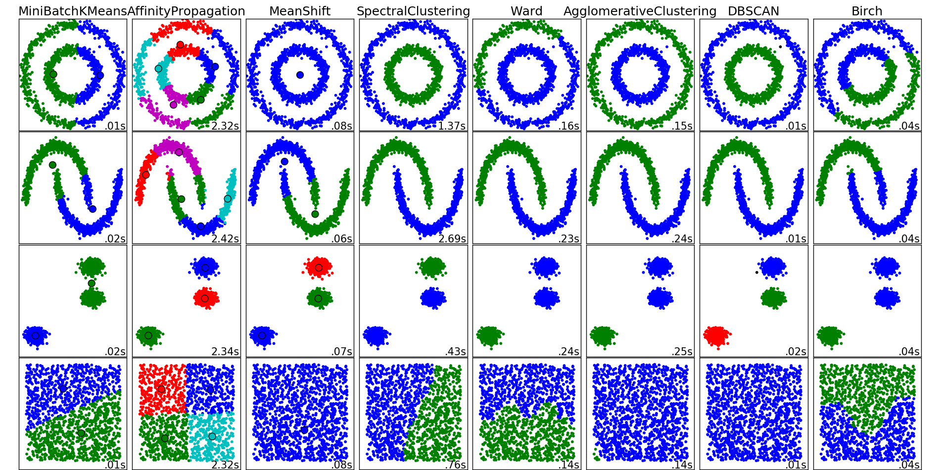
10.1.7. Porównanie algorytmów

• http://hdbscan.readthedocs.io/en/latest/comparing_clustering_algorithms.html

Porównanie algorytmów klastrowania

import time

import numpy as np
import matplotlib.pyplot as plt

from sklearn import cluster, datasets
from sklearn.neighbors import kneighbors_graph
from sklearn.preprocessing import StandardScaler

np.random.seed(0)

# Generate datasets. We choose the size big enough to see the scalability
# of the algorithms, but not too big to avoid too long running times
n_samples = 1500
noisy_circles = datasets.make_circles(n_samples=n_samples, factor=.5,
                                      noise=.05)
noisy_moons = datasets.make_moons(n_samples=n_samples, noise=.05)
blobs = datasets.make_blobs(n_samples=n_samples, random_state=8)
no_structure = np.random.rand(n_samples, 2), None

colors = np.array([x for x in 'bgrcmykbgrcmykbgrcmykbgrcmyk'])
colors = np.hstack([colors] * 20)

clustering_names = [
    'MiniBatchKMeans', 'AffinityPropagation', 'MeanShift',
    'SpectralClustering', 'Ward', 'AgglomerativeClustering',
    'DBSCAN', 'Birch']

plt.figure(figsize=(len(clustering_names) * 2 + 3, 9.5))
plt.subplots_adjust(left=.02, right=.98, bottom=.001, top=.96, wspace=.05,
                    hspace=.01)

plot_num = 1

datasets = [noisy_circles, noisy_moons, blobs, no_structure]
for i_dataset, dataset in enumerate(datasets):
    X, y = dataset
    # normalize dataset for easier parameter selection
    X = StandardScaler().fit_transform(X)

    # estimate bandwidth for mean shift
    bandwidth = cluster.estimate_bandwidth(X, quantile=0.3)

    # connectivity matrix for structured Ward
    connectivity = kneighbors_graph(X, n_neighbors=10, include_self=False)
    # make connectivity symmetric
    connectivity = 0.5 * (connectivity + connectivity.T)

    # create clustering estimators
    ms = cluster.MeanShift(bandwidth=bandwidth, bin_seeding=True)
    two_means = cluster.MiniBatchKMeans(n_clusters=2)
    ward = cluster.AgglomerativeClustering(n_clusters=2, linkage='ward',
                                           connectivity=connectivity)
    spectral = cluster.SpectralClustering(n_clusters=2,
                                          eigen_solver='arpack',
                                          affinity="nearest_neighbors")
    dbscan = cluster.DBSCAN(eps=.2)
    affinity_propagation = cluster.AffinityPropagation(damping=.9,
                                                       preference=-200)

    average_linkage = cluster.AgglomerativeClustering(
        linkage="average", affinity="cityblock", n_clusters=2,
        connectivity=connectivity)

    birch = cluster.Birch(n_clusters=2)
    clustering_algorithms = [
        two_means, affinity_propagation, ms, spectral, ward, average_linkage,
        dbscan, birch]

    for name, algorithm in zip(clustering_names, clustering_algorithms):
        # predict cluster memberships
        t0 = time.time()
        algorithm.fit(X)
        t1 = time.time()
        if hasattr(algorithm, 'labels_'):
            y_pred = algorithm.labels_.astype(np.int)
        else:
            y_pred = algorithm.predict(X)

        # plot
        plt.subplot(4, len(clustering_algorithms), plot_num)
        if i_dataset == 0:
            plt.title(name, size=18)
        plt.scatter(X[:, 0], X[:, 1], color=colors[y_pred].tolist(), s=10)

        if hasattr(algorithm, 'cluster_centers_'):
            centers = algorithm.cluster_centers_
            center_colors = colors[:len(centers)]
            plt.scatter(centers[:, 0], centers[:, 1], s=100, c=center_colors)
        plt.xlim(-2, 2)
        plt.ylim(-2, 2)
        plt.xticks(())
        plt.yticks(())
        plt.text(.99, .01, ('%.2fs' % (t1 - t0)).lstrip('0'),
                 transform=plt.gca().transAxes, size=15,
                 horizontalalignment='right')
        plot_num += 1

plt.show()  # doctest: +SKIP

10.1.8. Przykład praktyczny

10.1.9. K-means Clustering dla zbioru Iris

import numpy as np
import matplotlib.pyplot as plt
# Though the following import is not directly being used, it is required
# for 3D projection to work
from mpl_toolkits.mplot3d import Axes3D

from sklearn.cluster import KMeans
from sklearn import datasets

np.random.seed(5)

centers = [[1, 1], [-1, -1], [1, -1]]
iris = datasets.load_iris()
X = iris.data
y = iris.target

estimators = [
    ('k_means_iris_8', KMeans(n_clusters=8)),
    ('k_means_iris_3', KMeans(n_clusters=3)),
    ('k_means_iris_bad_init', KMeans(n_clusters=3, n_init=1, init='random')),
]

fignum = 1
titles = ['8 clusters', '3 clusters', '3 clusters, bad initialization']

for name, est in estimators:
    fig = plt.figure(fignum, figsize=(4, 3))
    ax = Axes3D(fig, rect=[0, 0, .95, 1], elev=48, azim=134)
    est.fit(X)
    labels = est.labels_

    ax.scatter(X[:, 3], X[:, 0], X[:, 2],  c=labels.astype(np.float), edgecolor='k')

    ax.w_xaxis.set_ticklabels([])
    ax.w_yaxis.set_ticklabels([])
    ax.w_zaxis.set_ticklabels([])
    ax.set_xlabel('petal_width')
    ax.set_ylabel('sepal_length')
    ax.set_zlabel('petal_length')
    ax.set_title(titles[fignum - 1])
    ax.dist = 12
    fignum = fignum + 1

# Plot the ground truth
fig = plt.figure(fignum, figsize=(4, 3))
ax = Axes3D(fig, rect=[0, 0, .95, 1], elev=48, azim=134)

for name, label in [('Setosa', 0),
                    ('Versicolor', 1),
                    ('Virginica', 2)]:
    ax.text3D(X[y == label, 3].mean(),
              X[y == label, 0].mean(),
              X[y == label, 2].mean() + 2, name,
              horizontalalignment='center',
              bbox=dict(alpha=.2, edgecolor='w', facecolor='w'))

# Reorder the labels to have colors matching the cluster results
y = np.choose(y, [1, 2, 0]).astype(np.float)
ax.scatter(X[:, 3], X[:, 0], X[:, 2], c=y, edgecolor='k')

ax.w_xaxis.set_ticklabels([])
ax.w_yaxis.set_ticklabels([])
ax.w_zaxis.set_ticklabels([])
ax.set_xlabel('petal_width')
ax.set_ylabel('sepal_length')
ax.set_zlabel('petal_length')
ax.set_title('Ground Truth')
ax.dist = 12

plt.show()  # doctest: +SKIP

10.1.10. Assignments

10.1.10.1. Klastrowanie zbioru Iris

• Assignment: Klastrowanie zbioru Iris

• Complexity: medium

• Lines of code: 30 lines

• Time: 13 min

English:

TODO: English Translation

Run doctests - all must succeed

Polish:

1. Dla zbioru Iris dokonaj klastrowania za pomocą algorytmu KMeans z biblioteki sklearn.

2. Dla jakiego hiperparametru n_clusters osiągniemy największe accuracy?

3. Zwizualizuj graficznie rozwiązanie problemu

4. Uruchom doctesty - wszystkie muszą się powieść