10.1. Polynomials
10.1.1. Defining
>>> import numpy as np
Polynomial of degree three:
Ax^3 + Bx^2 + Cx^1 + D = 0
1x^3 + 2x^2 + 3x^1 + 4 = 0
>>> np.poly1d([1, 2, 3, 4])
poly1d([1, 2, 3, 4])
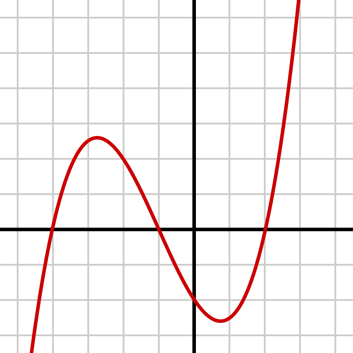
Figure 10.3. Polynomial of degree three Ax^3 + Bx^2 + Cx^1 + D = 0 [1]
Polynomial of degree six:
Ax^6 + Bx^5 + Cx^4 + Dx^3 + Ex^2 + Fx + G = 0
1x^6 + 2x^5 + 3x^4 + 4x^3 + 5x^2 + 6x + 7 = 0
>>> np.poly1d([1, 2, 3, 4, 5, 6, 7])
poly1d([1, 2, 3, 4, 5, 6, 7])
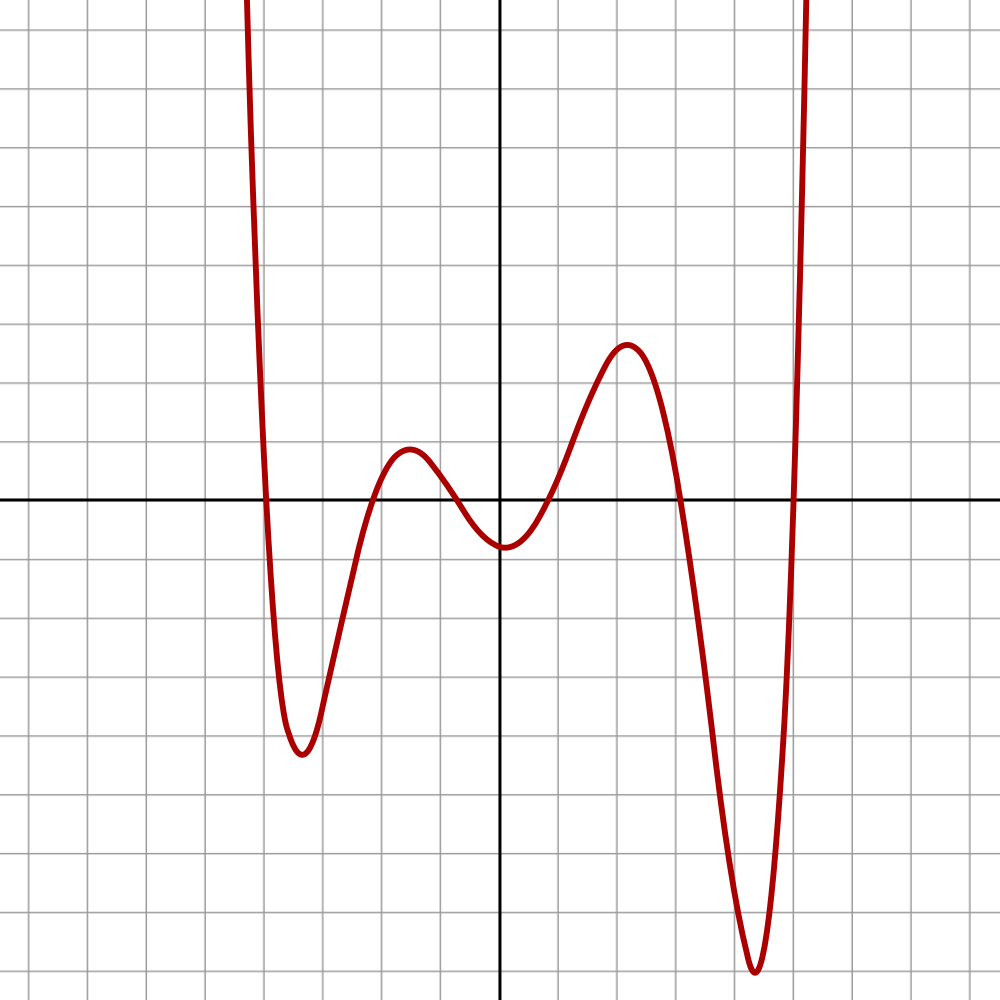
Figure 10.4. Polynomial of degree six Ax^6 + Bx^5 + Cx^4 + Dx^3 + Ex^2 + Fx + G = 0 [1]
10.1.2. Find Coefficients
Find the coefficients of a polynomial with the given sequence of roots
Specifying the roots of a polynomial still leaves one degree of freedom, typically represented by an undetermined leading coefficient.
>>> import numpy as np
>>> np.poly([0, 0, 0])
array([1., 0., 0., 0.])
>>> np.poly([1, 2])
array([ 1., -3.,  2.])
>>> np.poly([1, 2, 3, 4, 5, 6, 7])
array([ 1.0000e+00, -2.8000e+01,  3.2200e+02, -1.9600e+03,  6.7690e+03,
       -1.3132e+04,  1.3068e+04, -5.0400e+03])
10.1.3. Roots
Return the roots of a polynomial
>>> import numpy as np
>>> np.roots([1, 2])
array([-2.])
>>> np.roots([0, 1, 3])
array([-3.])
>>> np.roots([1, 4, -2, 3])
array([-4.5797401 +0.j        ,  0.28987005+0.75566815j,
        0.28987005-0.75566815j])
>>> np.roots([ 1, -11, 9, 11, -10])
array([10.+0.0000000e+00j, -1.+0.0000000e+00j,  1.+9.6357437e-09j,
        1.-9.6357437e-09j])
10.1.4. Derivative of a Polynomial
>>> import numpy as np
>>> np.polyder([1/4, 1/3, 1/2, 1, 0])
array([1., 1., 1., 1.])
>>> np.polyder([0.25, 0.33333333, 0.5, 1, 0])
array([1.        , 0.99999999, 1.        , 1.        ])
>>> np.polyder([1, 2, 3, 4])
array([3, 4, 3])
10.1.5. Antiderivative (indefinite integral) of a polynomial
Return an antiderivative (indefinite integral) of a polynomial
>>> import numpy as np
>>> np.polyint([1, 1, 1, 1])
array([0.25      , 0.33333333, 0.5       , 1.        , 0.        ])
>>> np.polyint([16, 9, 4, 2])
array([4., 3., 2., 2., 0.])
10.1.6. Evaluate a Polynomial at Specific Values
Compute polynomial values
Horner's scheme is used to evaluate the polynomial
>>> import numpy as np
>>> np.polyval([1, -2, 0, 2], 4)
34
10.1.7. Least Squares Polynomial Fit
Least squares polynomial fit
>>> import numpy as np
>>> x = [1, 2, 3, 4, 5, 6, 7, 8]
>>> y = [0, 2, 1, 3, 7, 10, 11, 19]
>>>
>>> np.polyfit(x, y, 2)
array([ 0.375     , -0.88690476,  1.05357143])
10.1.8. Polynomial Arithmetic
np.polyadd()np.polysub()np.polymul()np.polydiv()
10.1.9. Sum of Two Polynomials
>>> import numpy as np
>>> a = [1, 2]
>>> b = [9, 5, 4]
>>>
>>> np.polyadd(a, b)
array([9, 6, 6])
10.1.10. References
10.1.11. Assignments
"""
* Assignment: Numpy Polyfit
* Complexity: easy
* Lines of code: 4 lines
* Time: 8 min

English:
    1. Given are points coordinates in Cartesian system
    2. Separate first row (header) from data
    3. Calculate coefficients of best approximating polynomial of 3rd degree
    4. Run doctests - all must succeed

Polish:
    1. Dane są koordynaty punktów w układzie kartezjańskim
    2. Odseparuj pierwszy wiersz (nagłówek) do danych
    3. Oblicz współczynniki najlepiej dopasowanego wielomianu 3 stopnia
    4. Uruchom doctesty - wszystkie muszą się powieść

Tests:
    >>> import sys; sys.tracebacklimit = 0

    >>> assert result is not Ellipsis, \
    'Assign result to variable: `result`'
    >>> assert type(result) is np.ndarray, \
    'Variable `result` has invalid type, expected: np.ndarray'

    >>> result
    array([ 0.25,  0.75, -1.5 , -2.  ])
"""

import numpy as np

DATA = [
    ('x', 'y'),
    (-4.0, 0.0),
    (-3.0, 2.5),
    (-2.0, 2.0),
    (0.0, -2.0),
    (2.0, 0.0),
    (3.0, 7.0),
]


result = ...